SmolVLA: Asynchronous Inference

How SmolVLA makes the robot's brain think while its hands move — achieving 30% faster task completion
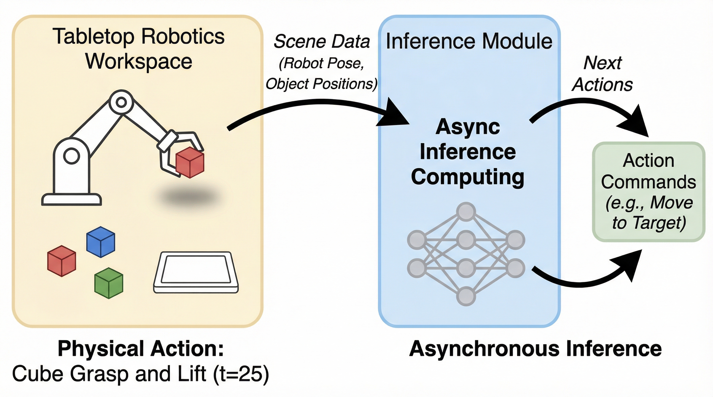
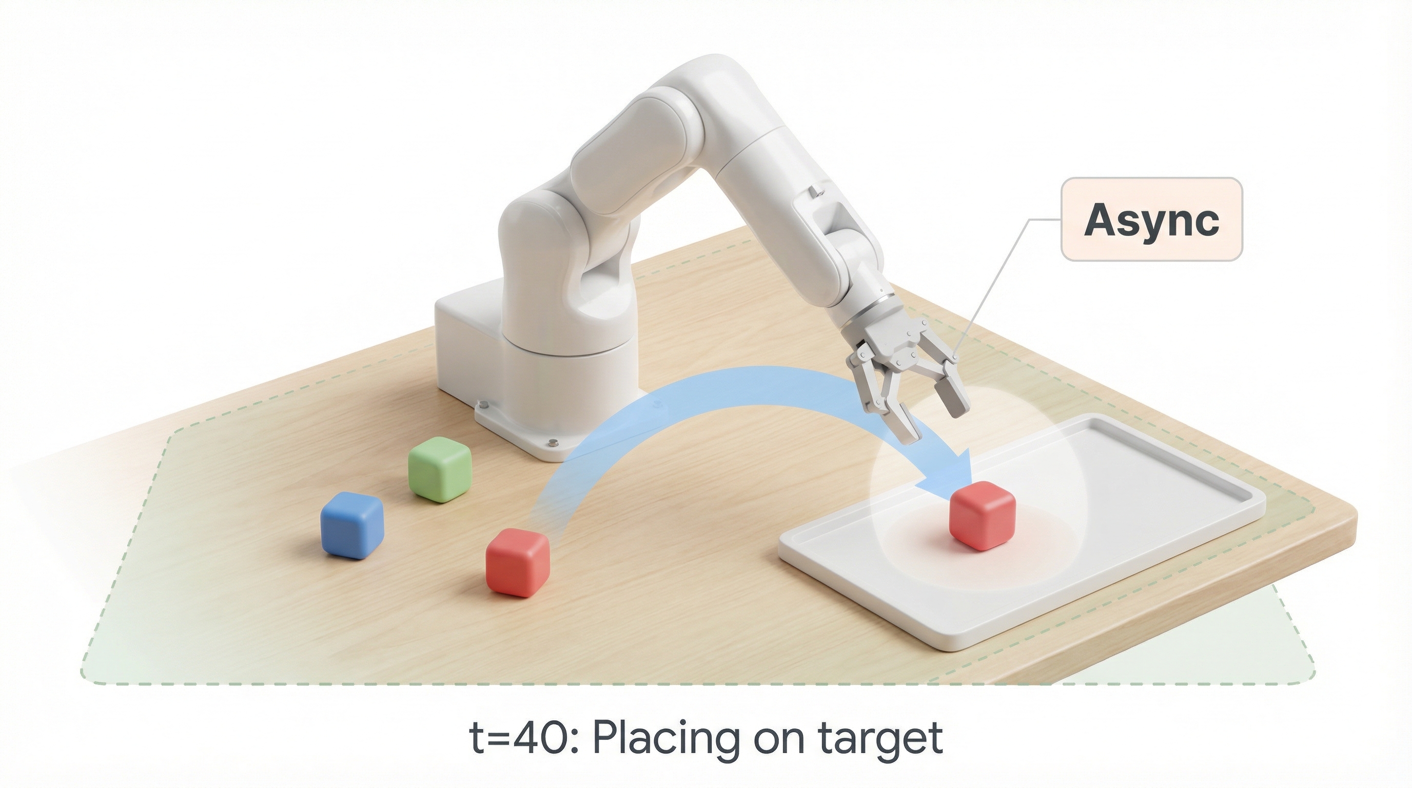
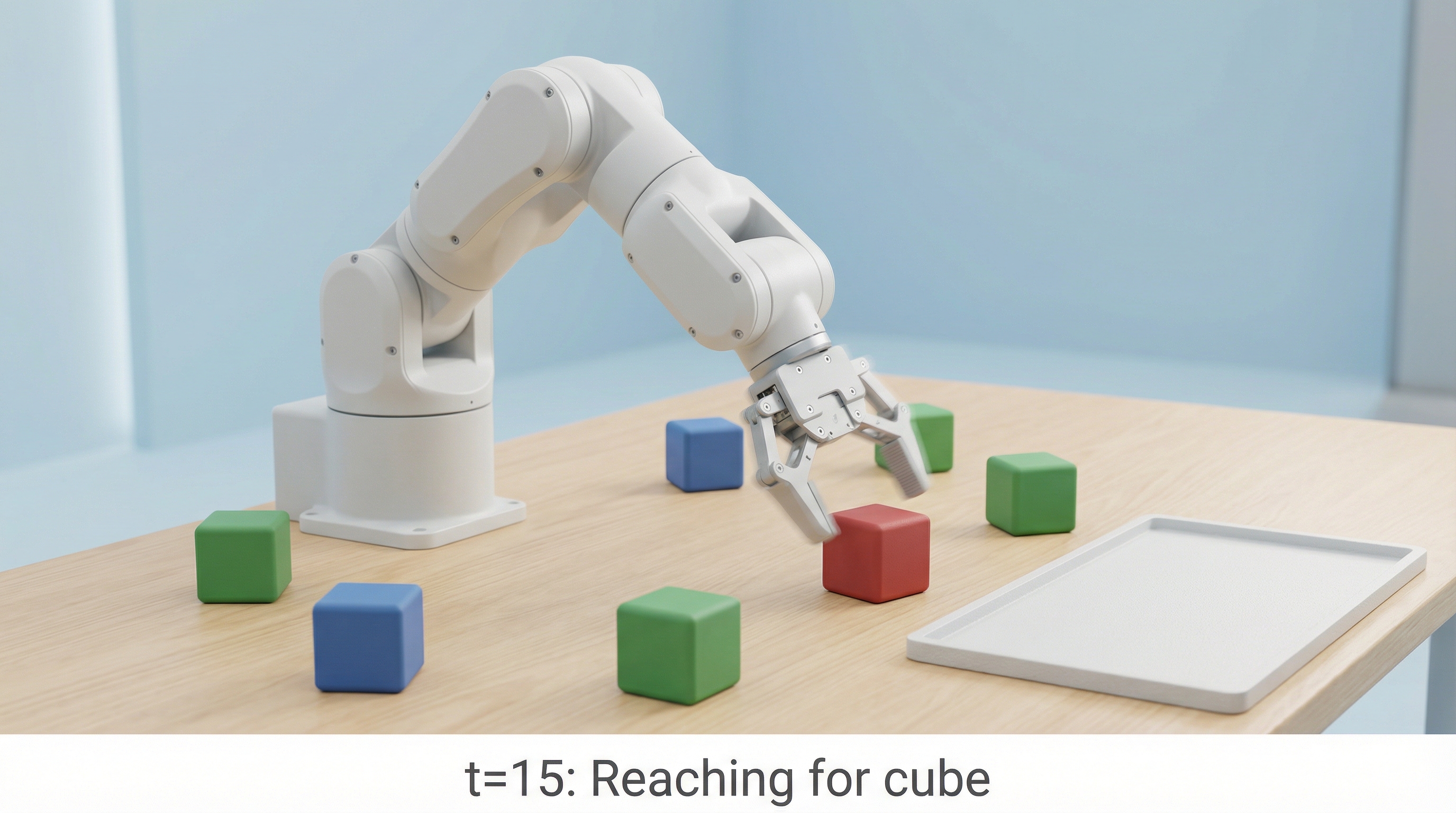
Robot picking up a cube

The Core Problem

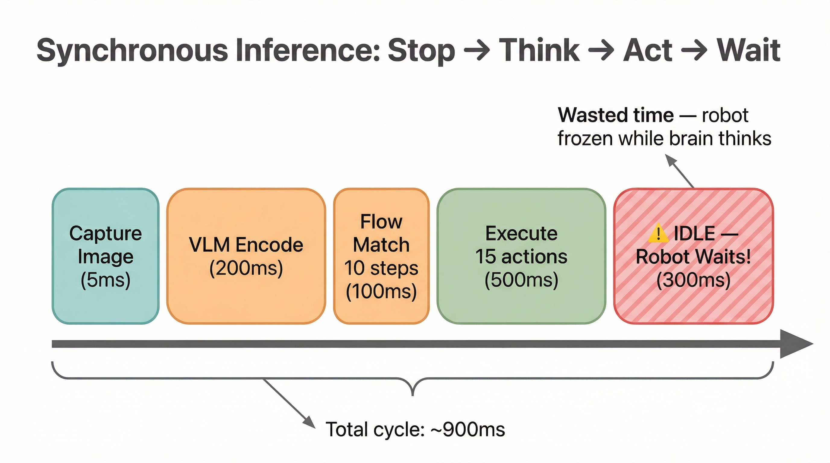
Vision-Language-Action models (VLAs) are slow. The VLM backbone needs ~200ms to process an image. The flow matching action expert needs another ~100ms for 10 denoising steps. During all that time, the robot just sits there waiting.

SmolVLA solves this with a simple but powerful idea: let the robot keep moving while the brain computes the next plan. This is asynchronous inference.

The Human Analogy

When you pour coffee, your hand is pouring while your eyes are already looking at where to set the mug down. You don't freeze your hand, look, plan, then resume. Your brain and hands work in parallel.

SmolVLA does exactly this — the robot executes the current batch of actions while the server is already computing the next batch from a fresh observation.
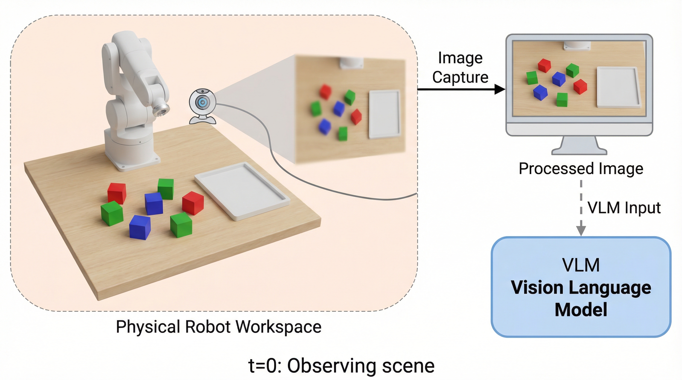
Observe
Observe
Reach
Reach
Pick
Pick
Place
Place

Step 1: The Synchronous Problem

Why running a VLA the naive way creates jerky, slow robot motion.

Synchronous pipeline

Interactive Synchronous Timeline

Watch one cycle of synchronous inference. Notice the red idle block — the robot is frozen while the VLM processes the next observation.

Capture Image (5ms)
VLM Encode (200ms)
Flow Match (100ms)
Execute Actions (500ms)
IDLE — Robot Frozen!
Press "Play Cycle" to see the synchronous pipeline in action.

The Numbers Tell the Story

Total cycle time = 5ms (capture) + 200ms (VLM) + 100ms (flow) + 500ms (execute) = 805ms Robot is IDLE for: 305ms out of every 805ms = 38% wasted time

Every cycle, the robot freezes for 300+ milliseconds. At 30 Hz control, that's ~9 missing frames of motion. The result: jerky, stop-and-go behavior that limits task success.

Step 2: Action Chunking Enables Async

The key insight: predicting many actions at once creates a buffer for parallel execution.

Why chunking enables async

Interactive: Single Action vs Action Chunk

Toggle between architectures to see why only chunked models can go async.

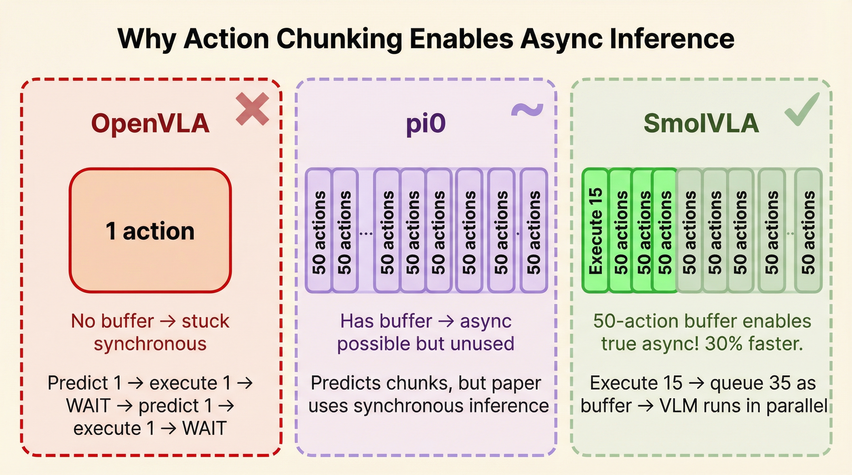
SmolVLA predicts 50 actions at once. While the robot executes actions from the buffer, the server is already computing the next 50. The action chunk is the bridge that decouples perception from execution.

OpenVLA

Predicts 1 action per inference.

No buffer — must wait for each action. Fundamentally synchronous. ~3 Hz effective control.

pi0

Predicts 50 actions per inference.

Has a buffer, but the paper uses synchronous inference. Async is possible in theory but not implemented.

SmolVLA

Predicts 50 actions + async execution.

Executes ~15 actions, queues the rest as buffer. VLM runs in parallel. 30% faster.

Step 3: Two-Process Architecture

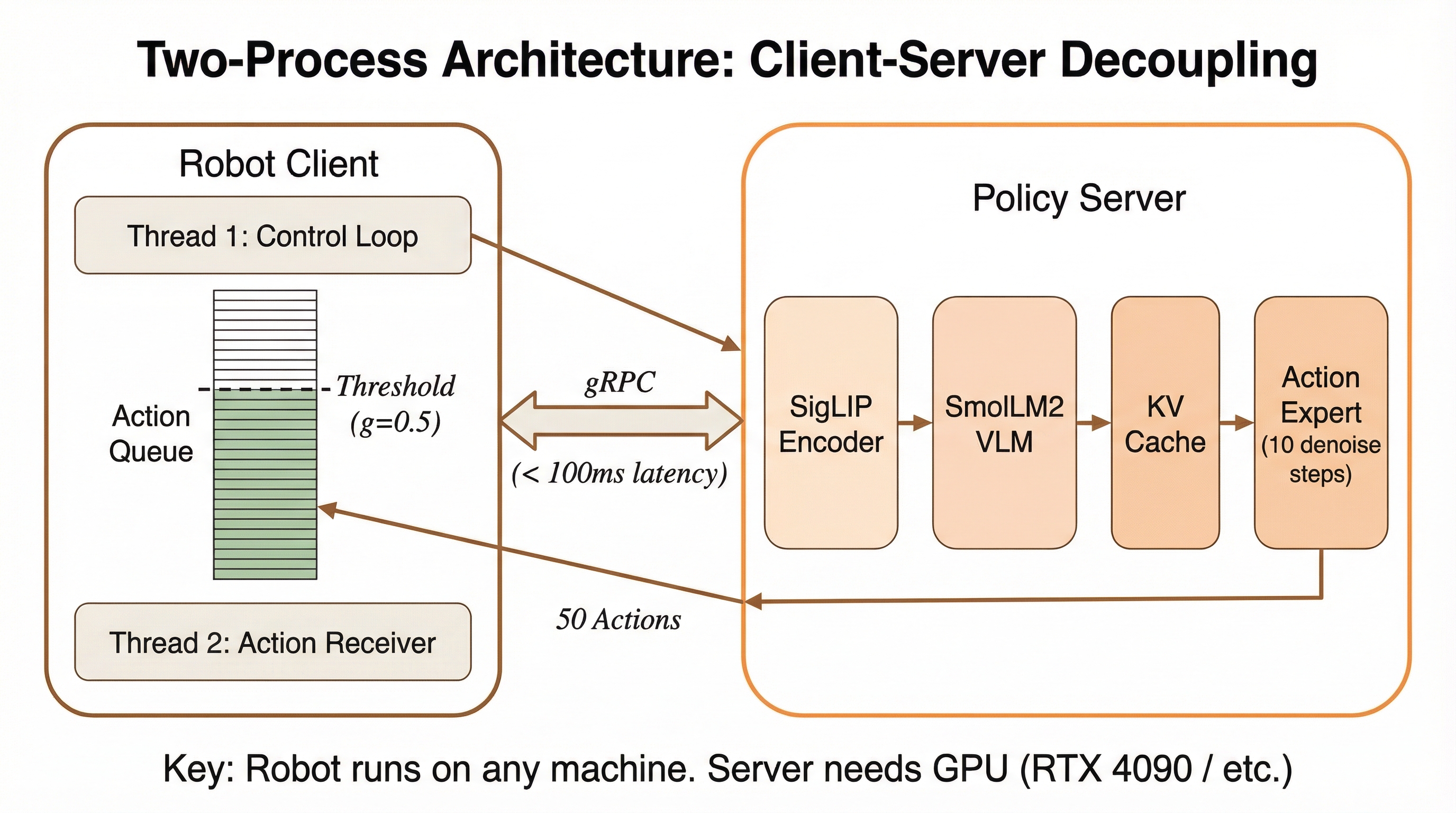
SmolVLA splits inference across a Robot Client and a GPU Policy Server, connected by gRPC.

Client-server architecture

Step-by-Step Walkthrough

1
2
3
4
5
6

Step 1: Robot Client captures observation

Thread 1 (Control Loop) captures a camera image + robot joint state. This becomes a TimedObservation with a timestamp.

obs = {image: cam.capture(), state: robot.get_state(), timestamp: now()}

The Two Threads

Thread 1: Control Loop

while running: action = queue.pop() robot.send_action(action) sleep(1/30) # 30 Hz if queue.size/50 <= 0.5: send_observation()

Thread 2: Action Receiver

while running: new_chunk = grpc.GetActions() with queue_lock: aggregate(queue, new_chunk) # 0.3*old + 0.7*new # for overlapping timesteps

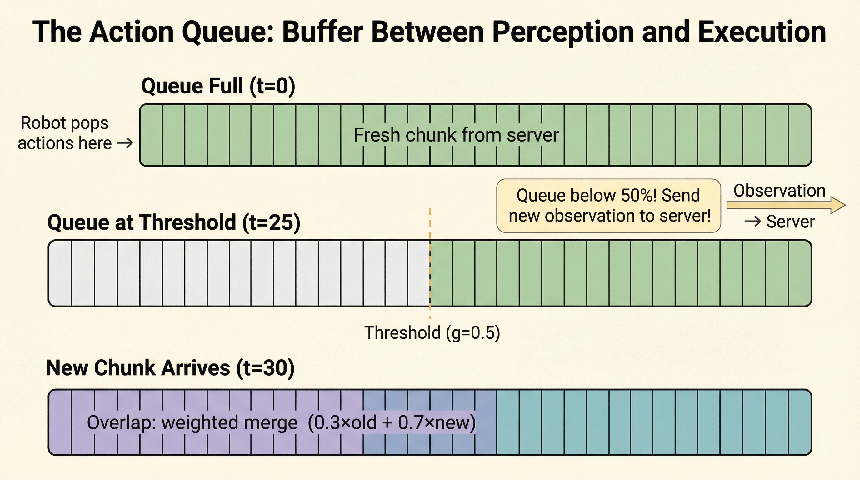
Step 4: The Action Queue

A FIFO buffer of future actions — the heartbeat of async inference.

Action queue mechanism

Interactive Queue Simulator

Watch the queue fill and drain in real time. When it drops below 50%, a new observation is sent to the server.

Robot pops actions → Queue: 50/50 actions ← Server pushes chunks
50% threshold (g=0.5)

Simulation log:

Ready. Press "Start Simulation".

Queue level over time

The Critical Threshold

Observation sent when: queue_size / chunk_size ≤ g   (g = 0.5 by default) At 50 actions and g=0.5: observation fires when 25 actions remain At 30 Hz: 25 actions = 833ms of buffer Inference takes ~300ms → 533ms of safety margin

As long as inference finishes before the queue empties, the robot never stops. If the queue ever does empty, a must_go flag forces immediate inference on the next observation.

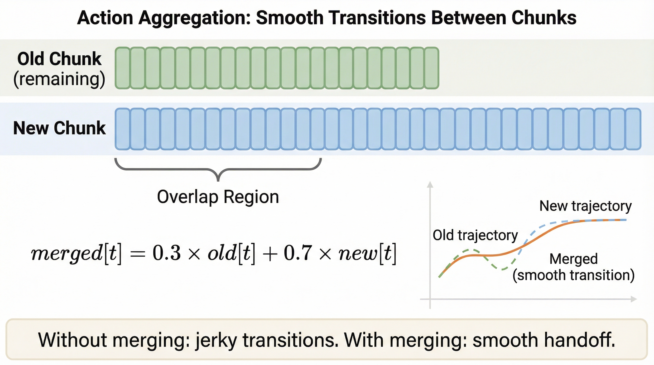
Step 5: Chunk Merging

When a new chunk arrives, it overlaps with remaining old actions. How do we blend them?

Chunk overlap merging

Interactive Aggregation Explorer

Adjust the weighting to see how old and new chunks blend in the overlap region.

Old chunk (remaining)
New chunk
Merged result

The Four Aggregation Strategies

AGGREGATE_FUNCTIONS = { "weighted_average": 0.3 * old + 0.7 * new, # default — trust new more "latest_only": new, # discard old completely "average": 0.5 * old + 0.5 * new, # equal blend "conservative": 0.7 * old + 0.3 * new, # trust old more (less reactive) }

The default weighted_average (0.3/0.7) works best: it trusts the newer prediction (computed from a more recent observation) while maintaining some continuity from the old trajectory, preventing jerky transitions.

Step 6: The Race — Sync vs Async

Watch two robots race to complete the same task. One runs synchronously, the other asynchronously.

Pick-and-Place Race

Both robots must pick up and place 5 cubes. The sync robot freezes during inference. The async robot never stops.

Sync Robot
S
0.0s
Async Robot
A
0.0s

Sync Robot Status

Cubes placed: 0/5

State: Waiting

Idle time: 0ms

Async Robot Status

Cubes placed: 0/5

State: Waiting

Queue level: 50/50

Side-by-Side Timeline

Detailed breakdown of what each robot is doing at every moment.

Executing actions
VLM + Flow Match
IDLE (robot frozen)
Overlap (execute + compute)

Step 7: The Results

Real-world experiments on SO-100 pick-and-place prove the async advantage.

Performance Comparison

13.7s

Synchronous
Average completion time

9.7s

Asynchronous
Average completion time

30%

Faster
Same success rate

Fixed-Time Throughput: The Real Story

In a fixed time budget, the async robot completed 19 cubes vs 9 cubes for synchronous — a 2.1x throughput improvement.

Technical Specifications

SmolVLA Model: Parameters: 450M (350M VLM + 100M Expert) Memory: ~2 GB (vs pi0: 14 GB) VLM backbone: SmolVLM-2 (500M → half layers) Vision encoder: SigLIP (64 tokens per image) Action expert: 10 flow-matching Euler steps
Async Inference: Communication: gRPC (< 100ms RTT) Chunk size: 50 actions Control freq: 30 Hz (33ms per action) Queue threshold: g = 0.5 (50%) Aggregation: 0.3×old + 0.7×new Server GPU: RTX 4090 (consumer!)

The Takeaway

Asynchronous inference is not a model improvement — it's an execution strategy. It works because action chunking provides the temporal buffer needed to decouple perception from execution. Any VLA that predicts action chunks can benefit from this approach.